Introduction to Pandas - Python Data Analysis Library#
Pandas - an external library for data analysis in Python.
It provides two basic data structures:
Series : a one-dimensional labeled array holding any type of data, even mixed data types.
DataFrame : a two-dimensional data structure that holds labeled data of any type.
In the following notebook, you will see some of the many functionalities of Pandas. This is not a data science course, and we recommend using the pandas documentation to see all the features.
Read more in the Pandas documentation
# First we need to import the pandas library as "pd"
import pandas as pd

# Numpy is still a very useful library, so we will also import that
import numpy as np
Intel MKL WARNING: Support of Intel(R) Streaming SIMD Extensions 4.2 (Intel(R) SSE4.2) enabled only processors has been deprecated. Intel oneAPI Math Kernel Library 2025.0 will require Intel(R) Advanced Vector Extensions (Intel(R) AVX) instructions.
Intel MKL WARNING: Support of Intel(R) Streaming SIMD Extensions 4.2 (Intel(R) SSE4.2) enabled only processors has been deprecated. Intel oneAPI Math Kernel Library 2025.0 will require Intel(R) Advanced Vector Extensions (Intel(R) AVX) instructions.
The Pandas Series#
# Creating a series directly from numbers (same type)
# which can be noted at the end of the print "dtype: int64"
a_series = pd.Series([1, 2, 5, 6, 8])
print("A series")
print(a_series)
A series
0    1
1    2
2    5
3    6
4    8
dtype: int64
# Creating a series directly from data (mixed types)
# which can be noted at the end of the print "dtype: object"
a_series = pd.Series([1, "mixed data", 5.5, np.nan, 8])
print("A series")
print(a_series)
A series
0             1
1    mixed data
2           5.5
3           NaN
4             8
dtype: object
# Creating a series using numpy functions
a_series = pd.Series(np.sin(np.linspace(1,6,10)))
print("A series")
print(a_series)
A series
0    0.841471
1    0.999884
2    0.857547
3    0.457273
4   -0.080542
5   -0.594131
6   -0.929015
7   -0.984464
8   -0.743802
9   -0.279415
dtype: float64
Functions to inspect the data#
Pandas offers a lot of functions to inspect or run data analysis directly on the Series or DataFrame (which we will see later in the notebook)
# Creating a series using numpy functions
a_series = pd.Series(np.linspace(0,10,11))
print("Print first 'n' elements using head(n=5). If no argument is given, default is 5 ")
print(a_series.head())

print()
print("describe() shows the basic statistics of the data")
print("but describe only gives numerical statistics, if all numbers are numeric")
a_series.describe()
Print first 'n' elements using head(n=5). If no argument is given, default is 5
0    0.0
1    1.0
2    2.0
3    3.0
4    4.0
dtype: float64

describe() shows the basic statistics of the data
but describe only gives numerical statistics, if all numbers are numeric
count    11.000000
mean      5.000000
std       3.316625
min       0.000000
25%       2.500000
50%       5.000000
75%       7.500000
max      10.000000
dtype: float64
# You can also describe mixed data, or a series of text
the_hobbit_beginning = pd.Series(["In","a","hole","in","the","ground","there","lived","a","hobbit.","Not","a","nasty,","dirty,","wet","hole,","filled","with","the","ends","of","worms","and","an","oozy","smell,","nor","yet","a","dry,","bare,","sandy","hole","with","nothing","in","it","to","sit","down","on","or","to","eat:","it","was","a","hobbit-hole,","and","that","means","comfort"])
the_hobbit_beginning.describe()
count     52
unique    41
top        a
freq       5
dtype: object
# or you can count words:
the_hobbit_beginning.value_counts()
a               5
hole            2
in              2
the             2
and             2
it              2
with            2
to              2
In              1
sit             1
bare,           1
sandy           1
nothing         1
on              1
down            1
yet             1
or              1
eat:            1
was             1
hobbit-hole,    1
that            1
means           1
dry,            1
an              1
nor             1
dirty,          1
ground          1
there           1
lived           1
hobbit.         1
Not             1
nasty,          1
wet             1
smell,          1
hole,           1
filled          1
ends            1
of              1
worms           1
oozy            1
comfort         1
Name: count, dtype: int64
Pandas DataFrame : The workhorse of Pandas#
Pandas dataframe is a 2-dimensional array that, again, allows mixed data types. This object offers a lot of functions to describe, sort, search and analyse data. One advantage of the dataframe, is that the columns are named, just like we know from an excel spreadsheet.
You can read more about DataFrames here
# Let us start by creating a dataframe manually.
x = np.linspace(0, 10, 11)
squares = x*x
cos = np.cos(x)
sin = np.sin(x)

# Collect all the data in a dictionary (the keys becomes the column names)
data_dict = {"x" : x, "squares" : squares, "cos"  : cos, "sin" : sin}

# and create the dataframe
df = pd.DataFrame(data_dict)

# Let us see the values we just added
df.head()
| x | squares | cos | sin | |
|---|---|---|---|---|
| 0 | 0.0 | 0.0 | 1.000000 | 0.000000 |
| 1 | 1.0 | 1.0 | 0.540302 | 0.841471 |
| 2 | 2.0 | 4.0 | -0.416147 | 0.909297 |
| 3 | 3.0 | 9.0 | -0.989992 | 0.141120 |
| 4 | 4.0 | 16.0 | -0.653644 | -0.756802 |
CSV dataset#
Let us take a look at a dataset from Kaggle: Used car sales data
In the following cells, we will investigate the “cars_df”, so remember to run the next cell before skipping.
# Start by reading the csv file (Note: pandas' read_csv is much faster than Numpy's)
cars_df = pd.read_csv("cars.csv")

# Let us investigate the data a bit
cars_df.head()
| Car_ID | Brand | Model | Year | Kilometers_Driven | Fuel_Type | Transmission | Owner_Type | Mileage | Engine | Power | Seats | Price | |
|---|---|---|---|---|---|---|---|---|---|---|---|---|---|
| 0 | 1 | Toyota | Corolla | 2018 | 50000 | Petrol | Manual | First | 15 | 1498 | 108 | 5 | 800000 |
| 1 | 2 | Honda | Civic | 2019 | 40000 | Petrol | Automatic | Second | 17 | 1597 | 140 | 5 | 1000000 |
| 2 | 3 | Ford | Mustang | 2017 | 20000 | Petrol | Automatic | First | 10 | 4951 | 395 | 4 | 2500000 |
| 3 | 4 | Maruti | Swift | 2020 | 30000 | Diesel | Manual | Third | 23 | 1248 | 74 | 5 | 600000 |
| 4 | 5 | Hyundai | Sonata | 2016 | 60000 | Diesel | Automatic | Second | 18 | 1999 | 194 | 5 | 850000 |
# We can also inspect what data types our dataframe holds
cars_df.info()
<class 'pandas.core.frame.DataFrame'>
RangeIndex: 100 entries, 0 to 99
Data columns (total 13 columns):
 #   Column             Non-Null Count  Dtype
---  ------             --------------  -----
 0   Car_ID             100 non-null    int64
 1   Brand              100 non-null    object
 2   Model              100 non-null    object
 3   Year               100 non-null    int64
 4   Kilometers_Driven  100 non-null    int64
 5   Fuel_Type          100 non-null    object
 6   Transmission       100 non-null    object
 7   Owner_Type         100 non-null    object
 8   Mileage            100 non-null    int64
 9   Engine             100 non-null    int64
 10  Power              100 non-null    int64
 11  Seats              100 non-null    int64
 12  Price              100 non-null    int64
dtypes: int64(8), object(5)
memory usage: 10.3+ KB
# Let us start by checking what "Brand"s there are in this dataset

# We can index a column directly as an attribute of the dataframe, here the "Brand"
# and then use the unique() method
cars_df.Brand.unique()
array(['Toyota', 'Honda', 'Ford', 'Maruti', 'Hyundai', 'Tata', 'Mahindra',
       'Volkswagen', 'Audi', 'BMW', 'Mercedes'], dtype=object)
# If we then wants to find the price range of each of these Brands
# then we can group all the products, then extract the "Price" of the products and statistically describe the data
cars_df.groupby("Brand")["Price"].describe()
| count | mean | std | min | 25% | 50% | 75% | max | |
|---|---|---|---|---|---|---|---|---|
| Brand | ||||||||
| Audi | 10.0 | 2.570000e+06 | 516505.351161 | 1900000.0 | 2050000.0 | 2600000.0 | 3000000.0 | 3200000.0 |
| BMW | 10.0 | 3.030000e+06 | 302030.167735 | 2700000.0 | 2800000.0 | 2900000.0 | 3200000.0 | 3500000.0 |
| Ford | 11.0 | 1.468182e+06 | 881269.745104 | 550000.0 | 675000.0 | 1500000.0 | 2250000.0 | 2700000.0 |
| Honda | 6.0 | 8.083333e+05 | 120069.424362 | 650000.0 | 750000.0 | 800000.0 | 850000.0 | 1000000.0 |
| Hyundai | 11.0 | 7.136364e+05 | 173336.247062 | 450000.0 | 550000.0 | 800000.0 | 850000.0 | 850000.0 |
| Mahindra | 5.0 | 9.400000e+05 | 250998.007960 | 700000.0 | 700000.0 | 900000.0 | 1200000.0 | 1200000.0 |
| Maruti | 6.0 | 7.083333e+05 | 80104.098938 | 600000.0 | 700000.0 | 700000.0 | 700000.0 | 850000.0 |
| Mercedes | 10.0 | 2.880000e+06 | 625033.332444 | 2300000.0 | 2425000.0 | 2700000.0 | 2900000.0 | 4000000.0 |
| Tata | 11.0 | 7.954545e+05 | 402774.468813 | 500000.0 | 500000.0 | 600000.0 | 1025000.0 | 1600000.0 |
| Toyota | 10.0 | 1.490000e+06 | 678560.568000 | 650000.0 | 950000.0 | 1400000.0 | 1800000.0 | 2500000.0 |
| Volkswagen | 10.0 | 1.115000e+06 | 559290.224799 | 500000.0 | 650000.0 | 1125000.0 | 1600000.0 | 1800000.0 |
# Now we can try and create a correlation matrix, that is, a matrix that give indications on whether or not
# variables are correlated. From intuition, we would think there should be a negative correlation between how old a car is
# and what sales value it should have. Meaning, the higher the age, the lower the price.

# Read more at e.g. : https://builtin.com/data-science/correlation-matrix
# Remember we have mixed data types, so we must provide the "numeric_only=True" argument
cars_df.corr(numeric_only=True)
| Car_ID | Year | Kilometers_Driven | Mileage | Engine | Power | Seats | Price | |
|---|---|---|---|---|---|---|---|---|
| Car_ID | 1.000000 | 0.059904 | -0.227442 | 0.026140 | -0.027965 | 0.027637 | -0.021582 | 0.037105 |
| Year | 0.059904 | 1.000000 | -0.741176 | 0.213177 | -0.355122 | -0.249446 | -0.252598 | -0.232687 |
| Kilometers_Driven | -0.227442 | -0.741176 | 1.000000 | -0.104437 | 0.112340 | -0.026732 | 0.396443 | -0.051104 |
| Mileage | 0.026140 | 0.213177 | -0.104437 | 1.000000 | -0.680949 | -0.648894 | -0.194581 | -0.595252 |
| Engine | -0.027965 | -0.355122 | 0.112340 | -0.680949 | 1.000000 | 0.805709 | 0.179179 | 0.714465 |
| Power | 0.027637 | -0.249446 | -0.026732 | -0.648894 | 0.805709 | 1.000000 | -0.102867 | 0.856620 |
| Seats | -0.021582 | -0.252598 | 0.396443 | -0.194581 | 0.179179 | -0.102867 | 1.000000 | -0.000027 |
| Price | 0.037105 | -0.232687 | -0.051104 | -0.595252 | 0.714465 | 0.856620 | -0.000027 | 1.000000 |
As seen from the matrix above, there is a clear correlation between Engine/Power and Price, and a negative correlation for year. But year is the absolute purchase yeah, not the age. So let us add a column for age, where “now” is 2024
# There are 2 ways to do this, you can a) provide a function or b) give a "lambda" expression.
# We will go with the lambda. axis=1 means loop over rows

# column "age" is now the result of each row's year being subtracted from 2024
cars_df['age'] = cars_df.apply(lambda row: 2024 - row.Year, axis=1)

# And now let us run the same correlation matrix
cars_df.corr(numeric_only=True)
| Car_ID | Year | Kilometers_Driven | Mileage | Engine | Power | Seats | Price | age | |
|---|---|---|---|---|---|---|---|---|---|
| Car_ID | 1.000000 | 0.059904 | -0.227442 | 0.026140 | -0.027965 | 0.027637 | -0.021582 | 0.037105 | -0.059904 |
| Year | 0.059904 | 1.000000 | -0.741176 | 0.213177 | -0.355122 | -0.249446 | -0.252598 | -0.232687 | -1.000000 |
| Kilometers_Driven | -0.227442 | -0.741176 | 1.000000 | -0.104437 | 0.112340 | -0.026732 | 0.396443 | -0.051104 | 0.741176 |
| Mileage | 0.026140 | 0.213177 | -0.104437 | 1.000000 | -0.680949 | -0.648894 | -0.194581 | -0.595252 | -0.213177 |
| Engine | -0.027965 | -0.355122 | 0.112340 | -0.680949 | 1.000000 | 0.805709 | 0.179179 | 0.714465 | 0.355122 |
| Power | 0.027637 | -0.249446 | -0.026732 | -0.648894 | 0.805709 | 1.000000 | -0.102867 | 0.856620 | 0.249446 |
| Seats | -0.021582 | -0.252598 | 0.396443 | -0.194581 | 0.179179 | -0.102867 | 1.000000 | -0.000027 | 0.252598 |
| Price | 0.037105 | -0.232687 | -0.051104 | -0.595252 | 0.714465 | 0.856620 | -0.000027 | 1.000000 | 0.232687 |
| age | -0.059904 | -1.000000 | 0.741176 | -0.213177 | 0.355122 | 0.249446 | 0.252598 | 0.232687 | 1.000000 |
In this dataset, age is not directly impacting the price. But the age has a strong correlation with kilometers driven, which makes sense, and a small negative correlation with Mileage, which also makes sense that newer cars tend to drive longer.
Sorry - not a data science course, but still fun! :-)
Quering data from a dataframe#
Let us try and look into some of the querying methods of Pandas DataFrames, still using the cars dataset. Here quering refers to selecting a subset of the dataframe.
# A subset of all the cars could be to find all "Fords"
ford_df = cars_df[cars_df.Brand == "Ford"]
ford_df.head()
| Car_ID | Brand | Model | Year | Kilometers_Driven | Fuel_Type | Transmission | Owner_Type | Mileage | Engine | Power | Seats | Price | age | |
|---|---|---|---|---|---|---|---|---|---|---|---|---|---|---|
| 2 | 3 | Ford | Mustang | 2017 | 20000 | Petrol | Automatic | First | 10 | 4951 | 395 | 4 | 2500000 | 7 |
| 11 | 12 | Ford | Endeavour | 2017 | 35000 | Diesel | Automatic | Second | 12 | 2198 | 158 | 7 | 2000000 | 7 |
| 21 | 22 | Ford | Figo | 2020 | 15000 | Petrol | Manual | Third | 18 | 1194 | 94 | 5 | 550000 | 4 |
| 30 | 31 | Ford | Aspire | 2019 | 26000 | Petrol | Manual | Third | 20 | 1194 | 94 | 5 | 600000 | 5 |
| 40 | 41 | Ford | Ranger | 2017 | 38000 | Diesel | Manual | Second | 12 | 2198 | 158 | 5 | 1500000 | 7 |
# or let us only see cars sold before 2020
older_cars_df = cars_df[cars_df.Year < 2020]
older_cars_df.head()
| Car_ID | Brand | Model | Year | Kilometers_Driven | Fuel_Type | Transmission | Owner_Type | Mileage | Engine | Power | Seats | Price | age | |
|---|---|---|---|---|---|---|---|---|---|---|---|---|---|---|
| 0 | 1 | Toyota | Corolla | 2018 | 50000 | Petrol | Manual | First | 15 | 1498 | 108 | 5 | 800000 | 6 |
| 1 | 2 | Honda | Civic | 2019 | 40000 | Petrol | Automatic | Second | 17 | 1597 | 140 | 5 | 1000000 | 5 |
| 2 | 3 | Ford | Mustang | 2017 | 20000 | Petrol | Automatic | First | 10 | 4951 | 395 | 4 | 2500000 | 7 |
| 4 | 5 | Hyundai | Sonata | 2016 | 60000 | Diesel | Automatic | Second | 18 | 1999 | 194 | 5 | 850000 | 8 |
| 5 | 6 | Tata | Nexon | 2019 | 35000 | Petrol | Manual | First | 17 | 1198 | 108 | 5 | 750000 | 5 |
# It is also possible to extract specific columns from the dataset
# Note two [[ ]] when having multiple columns, if a single column is needed, then ["Model"]
cars_df[["Model", "Price"]]
| Model | Price | |
|---|---|---|
| 0 | Corolla | 800000 |
| 1 | Civic | 1000000 |
| 2 | Mustang | 2500000 |
| 3 | Swift | 600000 |
| 4 | Sonata | 850000 |
| ... | ... | ... |
| 95 | C-Class | 2900000 |
| 96 | Innova Crysta | 1400000 |
| 97 | EcoSport | 750000 |
| 98 | Verna | 850000 |
| 99 | Altroz | 600000 |
100 rows × 2 columns
Plotting data from dataframes#
Let us finally see how we can plot data directly from dataframes.
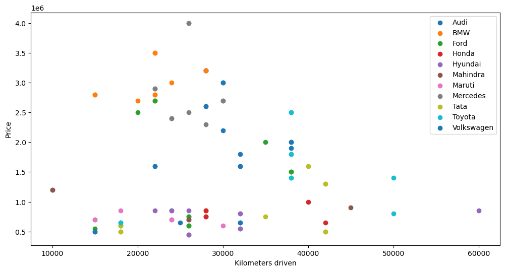
Note that we are using matplotlib as the plotting library in this case. Pandas has its own slim built-in plotting library. However the following example with multiple labels in a scatter plot is not straightforward in pure pandas.
import matplotlib.pyplot as plt
# We want to plot the kilometers driven on the X-axis and the Price on the Y-axis grouped by each Brand (color)

# Create the plot and axis
fig, ax = plt.subplots(figsize=(12,6))

# Loop over the groups of data
for name, group in cars_df.groupby('Brand'):
    ax.scatter(group.Kilometers_Driven, group.Price, label=name)

# Add legend and labels
plt.legend()
plt.xlabel("Kilometers driven")
plt.ylabel("Price")
Text(0, 0.5, 'Price')
Time series data : The weather in Stockholm#
Pandas has a lot of neat functions to work with time series data. Below we will revisit the weather data from the matplotlib workbook.
# Importing os to help with paths
import os
# First we need to read in the data. But since we have a 'date' field, we can tell pandas to treat it as such.
# The first column is a date:
date_cols = ['date']

# using the date_cols, we can tell pandas to convert into datetimes by using the 'parse_dates' argument
weather_df = pd.read_csv(os.path.join("..","matplotlib", "stockholm_daily_mean_avg_std_temperature.csv"), parse_dates=date_cols)

# Let us investigate the data a bit  - and we can see that the date field is now a datetime
weather_df.info()
<class 'pandas.core.frame.DataFrame'>
RangeIndex: 45132 entries, 0 to 45131
Data columns (total 4 columns):
 #   Column      Non-Null Count  Dtype
---  ------      --------------  -----
 0   date        45132 non-null  datetime64[ns]
 1   mean        45132 non-null  float64
 2   avg_toy     45132 non-null  float64
 3   stddev_toy  45132 non-null  float64
dtypes: datetime64[ns](1), float64(3)
memory usage: 1.4 MB
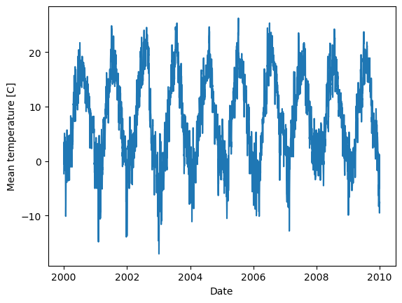
# Let's extract 2000 to 2010
# 'date' is the column name
sub_df = weather_df[weather_df['date'].between('2000-01-01', '2010-01-01')]
sub_df.head()
| date | mean | avg_toy | stddev_toy | |
|---|---|---|---|---|
| 36524 | 2000-01-01 | -2.3 | -2.23 | 4.96 |
| 36525 | 2000-01-02 | 1.3 | -1.78 | 4.57 |
| 36526 | 2000-01-03 | 0.8 | -1.93 | 4.55 |
| 36527 | 2000-01-04 | 3.5 | -2.35 | 4.83 |
| 36528 | 2000-01-05 | -0.6 | -2.78 | 5.00 |
# Now lets plot the mean temperature
plt.plot(sub_df['date'], sub_df['mean'])
plt.xlabel("Date")
plt.ylabel("Mean temperature [C]")
Text(0, 0.5, 'Mean temperature [C]')
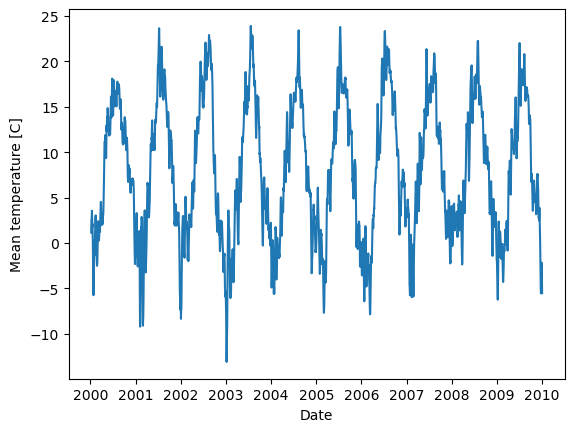
# We can also create a rolling mean of e.g. 7 days.

# each row in the data frame is one day, so that is just a rolling mean of 7 rows:
sub_df.loc[:,'weekly_mean'] = sub_df['mean'].rolling(7).mean()

# Now let's see what data we have
sub_df.info()

# and plot it using the mean
plt.plot(sub_df['date'], sub_df['weekly_mean'])
plt.xlabel("Date")
plt.ylabel("Mean temperature [C]")
<class 'pandas.core.frame.DataFrame'>
Index: 3654 entries, 36524 to 40177
Data columns (total 5 columns):
 #   Column       Non-Null Count  Dtype
---  ------       --------------  -----
 0   date         3654 non-null   datetime64[ns]
 1   mean         3654 non-null   float64
 2   avg_toy      3654 non-null   float64
 3   stddev_toy   3654 non-null   float64
 4   weekly_mean  3648 non-null   float64
dtypes: datetime64[ns](1), float64(4)
memory usage: 171.3 KB
/var/folders/0t/hldwbyfj7ls81tng6gt60p7r0000gn/T/ipykernel_98543/1679289622.py:4: SettingWithCopyWarning:
A value is trying to be set on a copy of a slice from a DataFrame.
Try using .loc[row_indexer,col_indexer] = value instead

See the caveats in the documentation: https://pandas.pydata.org/pandas-docs/stable/user_guide/indexing.html#returning-a-view-versus-a-copy
  sub_df.loc[:,'weekly_mean'] = sub_df['mean'].rolling(7).mean()
Text(0, 0.5, 'Mean temperature [C]')
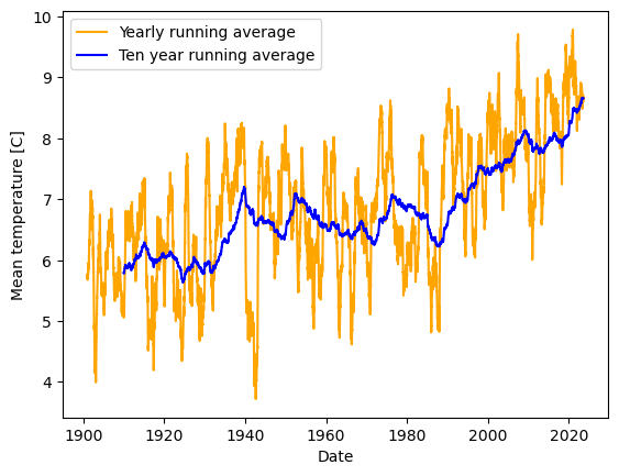
# Imagine if we instead want to see the yearly mean on all the data
weather_df.loc[:,'yearly_mean'] = weather_df['mean'].rolling(365).mean()
weather_df.loc[:,'ten_year_mean'] = weather_df['mean'].rolling(3650).mean()

plt.plot(weather_df['date'], weather_df['yearly_mean'], 'orange', label="Yearly running average")
plt.plot(weather_df['date'], weather_df['ten_year_mean'], 'b', label="Ten year running average")
plt.xlabel("Date")
plt.ylabel("Mean temperature [C]")
plt.legend(loc="upper left")
<matplotlib.legend.Legend at 0x7f77bb66edc0>